Random generation of problems

RAFF.jl contains several methods for the generation of artificial datasets, in order to simulate noisy data with outliers. See the API for details about the possibilities of random generation of data with outliers.

Simple example - the exponential function

First, it is necessary to load RAFF.jl and the desired model to generate the problem.

julia> using RAFF

julia> n, model, = RAFF.model_list["expon"]
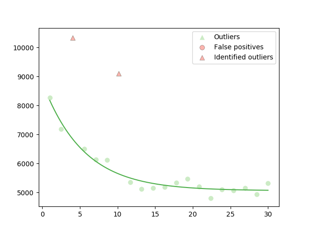
(3, getfield(RAFF, Symbol("##6#12"))(), "(x, θ) -> θ[1] + θ[2] * exp(- θ[3] * x[1])")

If an exact solution is not provided, RAFF.jl will generate a random one, but this can destroy the shape of some models. Therefore, in this example, we will provide a hint for a nice exponential model. In this example, we will generate 20 random points with 2 outliers in the interval $[1, 30]$.

julia> exact_sol = [5000.0, 4000.0, 0.2]
3-element Array{Float64,1}:
 5000.0
 4000.0
    0.2

julia> interv = (1.0, 30.0)
(1.0, 30.0)

julia> np = 20
20

julia> p = 18
18

Before calling the generating function, we fix the random seed, so this example is the same everywhere.

julia> using Random

julia> Random.seed!(12345678)
Random.MersenneTwister(UInt32[0x00bc614e], Random.DSFMT.DSFMT_state(Int32[485623157, 1073372256, 2105707176, 1072895099, -358862088, 1072969518, -2079238882, 1072755656, 281589009, 1073732136  …  1282907862, 1073649830, 1572678779, 1073436642, 124694191, -1919844179, -1265579980, 1299186829, 382, 0]), [0.0, 0.0, 0.0, 0.0, 0.0, 0.0, 0.0, 0.0, 0.0, 0.0  …  0.0, 0.0, 0.0, 0.0, 0.0, 0.0, 0.0, 0.0, 0.0, 0.0], UInt128[0x00000000000000000000000000000000, 0x00000000000000000000000000000000, 0x00000000000000000000000000000000, 0x00000000000000000000000000000000, 0x00000000000000000000000000000000, 0x00000000000000000000000000000000, 0x00000000000000000000000000000000, 0x00000000000000000000000000000000, 0x00000000000000000000000000000000, 0x00000000000000000000000000000000  …  0x00000000000000000000000000000000, 0x00000000000000000000000000000000, 0x00000000000000000000000000000000, 0x00000000000000000000000000000000, 0x00000000000000000000000000000000, 0x00000000000000000000000000000000, 0x00000000000000000000000000000000, 0x00000000000000000000000000000000, 0x00000000000000000000000000000000, 0x00000000000000000000000000000000], 1002, 0)

julia> data, = generate_noisy_data(model, n, np, p, x_interval=interv, θSol=exact_sol)
([1.0 8276.3 0.0; 2.52632 7187.67 0.0; … ; 28.4737 4944.13 0.0; 30.0 5322.83 0.0], [5000.0, 4000.0, 0.2], [7, 3])

Now we use the script test/script/draw.jl (see Advanced section) to visualize the data generated. draw.jl uses the PyPlot.jl package, so it is necessary to install it before running this example.

julia> include("test/scripts/draw.jl")

julia> draw_problem(data, model_str="expon")

If you are interested in running RAFF, just call the raff method. Attention: we have to drop the last column of data, since it contains information regarding the noise added to the outliers.

julia> r = raff(model, data[:, 1:end - 1], n, MAXMS=10)
** RAFFOutput **
Status (.status) = 1
Solution (.solution) = [5074.83, 6644.72, 0.691345]
Number of iterations (.iter) = 747
Number of trust points (.p) = 20
Objective function value (.f) = 2.0178898358722646e7
Number of function evaluations (.nf) = 747
Number of Jacobian evaluations (.nj) = 396
Index of outliers (.outliers) = Int64[]

If all the steps were successful, after command

julia> draw_problem(data, model_str="expon", raff_output=r)

the following picture should appear